

Outline
1. Developments of Remote Sensing
- Definition and Origin
- Early Developement
- Modern Era
2. Electromagnetic Spectrum
- Visible
- Ultra Violet to near Infrared
- Radar
3. Object Recognition
- People or Computers
- Variability of Reflectance due to Environmental Conditions
4. Photogrammetry
- Definition and Basic Concepts
- Kelsh Stereoplotter
- Analytical Stereoplotters
- Orthoscope
- Digital Orthoscope
5. Multispectral Pattern Recognition
- Definition
- Multiple Band Images
- Landsat Band Combinations
- Characteristic Reflectance Values
- Spectral Signature
- Image Classification Algorithm
- Probability Analysis
6. Sensors
- LANDSAT MSS
- LANDSAT TM
- SPOT
- QuickBird
- Ikonos
- Other Remote Sensing Sensors
7. Relationship with GIS
- Orthophoto Phenomenon
- Change Analysis
- Software Vendor Dominance
8. Questions
9. Additional Links
1. Developments of Remote Sensing
Definition and Origin
Generally speaking, Remote Sensing is the acquisition and analysis of information about objects or phenomena from a distance. In regards to the discipline of geography, it is the acquisition and analysis of information about the Earth (or other planetary bodies) through the use of computer and sensor systems via electromagnetic radiation. It could be argued that Remote Sensing originated with any human gaining a high perspective of an area, but in a more sophisticated sense it began in the 1830s with the invention of the camera. Major advancements were made during World War II with the development of RADAR (Radio Amplified Detection and Ranging) and SONAR (SOund NAvigation and Ranging). Side Looking Airborne Radar (SLAR) was also invented during World War II and its product is a high resolution image. Early Developement
In the Late 1950's, fixed wing aerial photography was extensively developed. In the early 1960's, the space race had begun between Russia and the United States. Image based satellite systems were developed, especially with regard to military spy satellites and civilian weather observation satellites. Radar and was vastly improved upon. Synthetic Aperture Radar (SAR) systems were developed was also developed during this time.
Modern Era
Remote sensing came of age in the 1970's with the refinement of satellite imaging. In 1972 the Earth Resources Technology Satellite (ERTS) was renamed to LANDSAT (NASA). The sensor had an 80 meter/pixel spatial resolution. In 1975, constant image download was available from LANDSAT, with an 18 day temporal resolution (passing over the same geographical area every 18 days). So much data became available, that Earth Resources Observation Systems (EROS) data center was established in South Dakota. Initial cost for four band (Red, Blue, Green and Infrared) LANDSAT scenes (approximately 100km x 100km area) averaged $200.
2. Electromagnetic Spectrum

Electromagnetic Spectrum
VisibleThe electromagnetic (EM) spectrum is the complete range of wavelengths of electromagnetic radiation emitted from the sun, ranging from the extremely short Gamma rays to the longer radio waves. The incident energy emitted from the sun is never destroyed; it is absorbed, reflected, or transmitted by an object. Of the total EM spectrum, visible light comprises a tiny sliver. The visible portion of the EM (.4 - .7 micrometers) is especially important in assessing the biomass (health of pigmentation) of vegetation. Healthy plants tend to have high chlorophyll content. In the visible spectrum, chlorophyll absorbs red and blue light and reflects green light. Greater chlorophyll content will result in an increased reflectance in the green portion of the EM, and producing a visual green appearance of a healthy plant.
Ultra Violet to near Infrared
Multispectral scanners can image from UV through the thermal IR band. The Near Infrared portion of the EM (.7 1.3 micrometers) is sensitive to leaf structure. The greatest amount of EM energy reflected the plants is in the Near IR. The variability in reflectance is associated with the mesophyll layer of plant leaves. Younger plants tend to have a well defined mesophyll layer resulting in higher Near IR reflectance. As leaves mature or is stressed by environmental influences (drought, disease), the mesophyll layer structure deteriorates. This results in a lower reflectance in of Near IR. Using this knowledge enables scientists to track the state of vegetation coverage without having to do field analysis. Most often in remote sensing images, healthy vegetation appears red.
Radar
Microwave wavelengths, from 1mm to approximately1 meter, have been imaged using RADAR, SLAR (Side Looking Airborne Radar), SAR (Synthetic Aperture Radar), SIR (Shuttle Imaging Radar), and SRTM (Shuttle Radar Topography Mission). Advantages of RADAR include the ability to penetrate cloud coverage and image surfaces in total darkness. Because of its ability to penetrate through clouds, RADAR has been used to map the surface of the planet Venus.
3. Object Recognition
People or Computers
Object identification through remote sensing applications is accomplished through identification of unique spectral response curves. Land Cover classification through remote sensing applications involves either unsupervised (computer generated) interpretation), or supervised (human interpretation) classification. Currently great strides have made in the arena of artificial intelligence to improve this process. Human interpretation, when combined with remote sensing applications is still the most effective classification tool.Variability of Reflectance due to Environmental Conditions
In performing a supervised classification, the representation of a single feature within an image is highly variable as a result of shadowing, terrain, moisture, atmospheric conditions, and sun angle.

4. Photogrammetry
Deffinition and Basic Concepts
Photogrammetry is the technique of measuring objects (2D or 3D) from photo-grammes (= photographs). Photogrammetric camera systems have automated film advance and exposure controls, as well as use long continuous rolls of film. Aerial photographs are taken in a continuous sequence with approximately 60% overlap. This overlap (conjugate) area of adjacent images enables 3 dimensional analysis for extraction of point elevations and contours. Parallax is the relative displacement of features on two overlapping photographs. Overlap can be as much as 60% in the vertical direction and 40% in the horizontal direction. Taking into account parallax, shadows on an image can be used to determine the heights of vertical features (buildings, trees, towers, cliffs, etc.), as well as the time of day.Kelsh Stereoplotter
Harry T. Kelsh introduced the Kelsh optical projection stereoplotter in 1945. This German photogrammetric instrument was used create a 3 dimensional image from overlapping analog images (conjugate images) for extracting precise elevation information (i.e. point elevations and contours). Accurate elevation measurements were derived by adjustment of a floating point. By placing the floating point to the perceived surface of the 3 dimensional image accurate point elevations or contours were derived. This is still a common method for creating topographic maps today.Analytical Stereoplotter
Analytical Stereoplotters combine capabilities of computer technology with stereoplotter functionality in order to limit operator intervention in the adjustment of parallax (the relative displacement of features on two overlapping photos). With most analytical stereoplotters, operator assistance is required for fine adjustment of parallax so that the floating dot in the visual field is placed directly on the 3 dimensional surface. There are 4 basic types of analytical plotters: anaglyphic, polarizing, stereo image alternators, stereo optical training, digital photometric (softcopy) workstations.
Anaglyphic stereoplotters pass each image through separate colored filters (red and blue-green) so that both images can be displayed on a single monitor. The operator is required to wear special colored glasses to view the 3 dimensional image.
Polarized stereoplotters pass light through polarized lenses so that the images are polarized in different directions. Both images are then displayed on a single monitor. The operator is required to wear special polarized glasses to view the 3 dimensional image.
Stereo image alternators change the view on the monitor between the 2 stereo images at a high frequency to create a false 3 dimensional image that can be viewed without the aid of glasses.
Stereo optical training passes light from each image through a series of mirrors and prisms to binocular type lenses. The operator views the stereo image through the binoculars.
Digital Photometric (softcopy) workstations view conjugate digital stereo models on a single computer monitor as a polarized image. The operator is required to wear special polarized glasses to view the 3 dimensional image.
Orthoscope
An orthoscope is an optical distortion device used to remove distortion from a photograph. When aerial photo is taken it has a central perspective. This means that it is being viewed downward at the central point causing distortion near the edge. To reduce the amount of distortion a planemetric perspective will be achieved. It is when a photo appears as though it is being looked at from straight above the earth at every point. A conversion will be made from a central to a planemetric perspective. This will be achieved by stretching the distortions.Digital Orthoscope
Today there is a different way to remove distortion from photos by digital alterations. This is accomplished by first scanning in the photographs to create a raster image. Pixels can then be removed or moved to eliminate distortion. This method provides a more efficient way to correct images.5. Multispectral Pattern Recognition
Definition
Using different regions of the electromagnetic spectrum to identify and to do analysis of remotely sensed features.Multiple Band Images
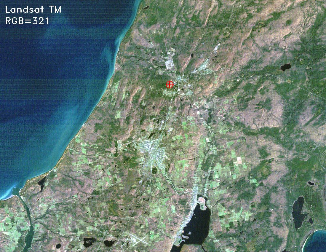
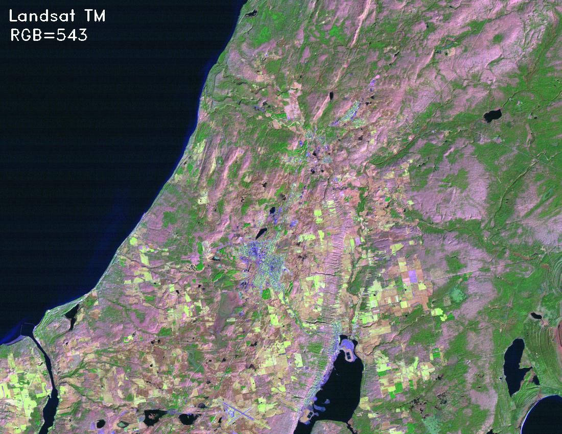
Remote sensing sensors (Landsat, SPOT, AVIRIS, AVHRR, LIDAR, SAR, etc.) record the relative brightness of an area over specific portions of the electromagnetic spectrum. All sensors have spectral sensitivity limitations; this is referred to as spectral resolution. No single sensor is sensitive to all wavelengths of the electromagnetic spectrum. Recorded wavelengths are referred to as bands. The number of bands varies depending on the sensor system (multispectral, hyperspectral, radar). Displaying of a remote sensing image on a computer monitor is limited to 3 bands. Selected bands are shown consecutively through the three color monitor guns (red, green, and blue). This produces a false image. Band color combinations are dependent upon the type of feature analysis being performed.LANDSAT TM Band Combinations
| Helpful Landsat TM Band Combinations | ||||
| | | | | |
| Red | Green | Blue | Feature | Screen color |
| 7 | 4 | 2 | Bare Soil | Magenta/Lavendar/Pink |
| | | | Crops | Green |
| | | | Urban Areas | Lavendar |
| | | | Wetland Vegetation | Green |
| | | | Trees | Green |
| 3 | 2 | 1 | Bare Soil | White/Light Grey |
| | | | Crops | Medium-Light Green |
| | | | Urban Areas | White/Light Grey |
| | | | Wetland Vegetation | Dark Green/Black |
| | | | Trees | Olive Green |
| 4 | 3 | 2 | Bare Soil | Blue/Grey |
| | | | Crops | Pink/Red |
| | | | Urban Areas | Blue/Grey |
| | | | Wetland Vegetation | Dark Red |
| | | | Trees | Red |
| 4 | 5 | 3 | Bare Soil | Green/Dark Blue |
| | | | Crops | Yellow/Tan |
| | | | Urban Areas | White/Blue |
| | | | Wetland Vegetation | Brown |
| | | | Trees | Tan/Orange Brown |
Characteristic Reflectance Values
Reflectance values are a result of "...energy reflected and emitted back from an object that is detected by a sensor. The measure of reflected energy is referred to a radiometric resolution. By analyzing energy received by the sensor, information about features can be derived." (Arnoff, p. 63). The energy that is reflected or emitted back represents characteristic of a feature at that particular moment. All features have unique reflectance characteristics. This is useful when identifying features represented within any type of image (pan chromatic, remotely sensed, or radar). Reflectance values can be easily imported into a GIS.Spectral Signature
At one time it was thought that each object had its own spectral signature. This would mean that a birch tree would have one reflectance value and a maple tree would have a totally separate reflectance value. In the 1970's it was realized that this could not be achieved for two main reasons: 1.there are a variety of factors that may change an objects reflectance patterns such seasonal changes, environmental moisture content, and 2. data format. When dealing with raster based information mixed pixels (mixels) are inevitable. All sensors have in inherent limitation to just how small of an object on the Earth s surface can be identified from its surroundings. The measure of size is referred to as spatial resolution. Spatial resolution reflects the smallest object that can be detected by a sensor. As an example, Landsat TM has a spatial resolution of 30 X 30 meters. The sum of all of the spectral reflectance of all features within the 30 X 30 meter footprint comprises a spectral response pattern that is detected by the sensor. If an operator want to identify features that are less then 30 X 30 meters, a different sensor with a resolution <30 meters must be selected. Image Classification Algorithm
Land cover classification from remotely sensed imagery that requires minimal operator input is referred to as unsupervised classification.
Land cover classification from remotely sensed imagery that requires significant operator input is referred to as supervised classification.
Probability Analysis
This is a program procedure that is based on probability analysis to identify or classify what features are. It is an image classification algorithm. When used it says there is a 60% (or whatever the percentage is) that the object is what it is. This value can be calculated by performing statistical measures and weighting the data. Today, probability analysis along with image classification algorithms are used to distinguish features and analyze data compared to when object recognition was the preferred method. This new method became known as multispectral pattern recognition; the different spectral responses are used to tell about the image versus the shape of features.6. Sensors
LANDSAT MSS
The first Landsat launched by the United Sates was on July 23, 1972. They were used in an effort to collect data about the earth's resources from a satellite as stated by Arnoff. The multi spectral scanner (MSS) provided digital images that could be used for computer analysis. It had four bands (4, 5, 6, and 7) in the visible and near infrared part of the spectrum. The sensor s spatial resolution was approximately 79m by 56m as stated by Arnoff. It also had a return orbit period of 18 days. The orbit was sun synchronous (in its orbital path, the satellite will always pass over a given location of the earth at the same local sun time).LANDSAT TM
Landsat TM is more advanced multispectral scanner than the MSS system. The spectral resolution encompasses seven bands that range from visible blue to thermal infrared. Included is a Mid Infrared (MIR) band. Please note band seven is out of the spectral sequence because it was added after band 6 had been developed. Not only does TM cover more of the spectrum, but it has a higher spatial resolution of 30m x 30m. Images may have a "true" or "false" color. True reflects actual surface colors seen by the human eye. False color results from selected band combinations being consecutively displayed on the color monitor through the red green blue (rgb) color guns. The features will not look like they do to the naked eye. In a Landsat 7 TM 4 (Infrared), 3 (red visible), 2 (green visible) color combination; the infrared band will be shown through the red gun, the red visible band will be shown through the green gun, and the green visible band will be shown through the blue gun. In this combination, healthy vegetation will appear red (not green) in the image.
SPOT
Systeme Pair l'Observation de la Terre (SPOT) started in France in 1978. It originated as a commercial program. SPOT has two HRV push broom scanners that can produce either a panchromatic (a single visible band black and white) with a 10 meter spatial resolution or a multi spectral 3 bands (2 visible, 1 infrared) with a 20 meter spatial resolution. The sensor orbit is sun synchronous with a 26 day nadir and 1-5 days off nadir temporal resolution. The sensor also has the capability to produce full scene stereo images which can be used to create topographic maps. SPOT 5, launched in 2002 has improved spatial resolution for both panchromatic (2.5 and 5 meter) and multispectral images (10 meter visible, 10 meter Near IR). Overall the Landsat TM has greater spectral resolution and SPOT has better spatial resolution.Quick Bird
The predecessor to QuickBird was the Early Bird Satellite system, developed by Earth Watch. Earth Watch, former in 1993, was a pioneer company in the privatization of high resolution satellite based image sources. In 2001 Earth Watch changed its name to Digital Globe.
The first EarlyBird satellite was launched by the Russians in December 1997. Though the launch was a success, the satellite failed to achieve the proper orbit. In April 1997, the satellite was declared a loss. In November 2000, QuickBird was launched at the Cosmodrome in Russian and failed to reach orbit. In October 2001 QuickBird 2 was successfully placed into orbit with the capability of .61 meter spatial resolution and 4 band (blue, green, red, NIR) spectral resolution. Both spatial and spectral resolutions are much improved over the EarlyBird sensor. Temporal resolution of the QuickBird is 1-4 days, depending on latitude (poles = 1 day, equator = 4 days). Data download locations include Norway, Alaska, and Colorado (company headquarters).
IKONOS
Ikonos was the first 1 meter spatial resolution commercial imaging satellite system to achive orbit. Ikonos 1, Launched in 1998, failed to achieve orbit. The 1999 launch of Ikonos 2 was a success. Ikonos 2 provides customers world-wide with 1 meter panchromatic and 4 meter multispectral imagery spatial resolution.
Other Remote Sensing Sensors
Past Remote Sensing Sensors
Current and Future Remote Sensing Sensors
Images from Other Remote Sensing Sensors
7. Relationship to GIS
Orthophoto PhenomenonOrthophotography first came into use in the 1960's, but they did not become commonplace until the 1970s due to cost. Digital Orthophotos are commonly used as a backdrop for vector digitizing. Orthophoto show the actual land feature of an area as opposed to the generalizations found on a map.
Change Analysis
Change analysis refers to the process of comparing changes to the same area using remotely-sensed images that are temporally separated. Change analysis developed in the 1970s at a time when GIS was in its early, developmental stages. Raster based data laid the ground-work for GIS and remote sensing analysis. "Vegetation indices" and Dana Tomlin's "Map Algebra" were developed in this era.Software Vendor Dominance
Prominent software vendors who have dominated the GIS and remote sensing arena are ESRI (vector based data display) and ERDAS (multi spectral data manipulation). ERDAS dominates the Remote Sensing market.


